Data Science Notes 6: Multiple linear regression

My earlier posts in this series:

• Data Science Notes 1, Introduction to machine learning
• Data Science Notes 2, Machine learning and Python
• Data Science Notes 3, Data preprocessing
• Data Science Notes 4, Feature scaling
• Data Science Notes 5, Linear regression

Hello. In my previous data science post I told you about linear regression. In this one I will talk about linear regression again, with a few differences. As in the earlier posts, the first thing I will do is explain the theory and then move to the Python application. I hope it is useful.

What is multiple linear regression?

To understand multiple linear regression you first have to understand linear regression, so let us look at the dataset I used in the previous post.

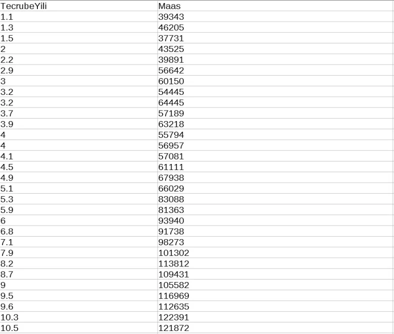
Looking at the dataset above we see two variables. One is dependent and one is independent. We found the relationship between them with linear regression, built a model and then tested it. But what do we do when linear regression involves more than one variable? This is where multiple linear regression comes in. Multiple linear regression is the method for finding the relationship between variables in datasets that depend on more than one variable and whose dependent variable increases linearly.

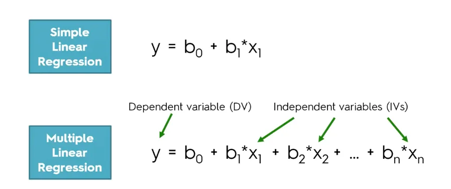
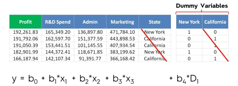
In multiple linear regression, each independent variable affects the dependent variable to a different degree. So compared with the equation in simple linear regression, the coefficients of the variables do not have to be the same. In the third post of this series I covered turning categorical attributes into numbers. There, the variable with categorical values had more than one kind of value (Hatay, Istanbul, Karaman), so we gave each one a number. For categorical variables with only two kinds of value we can use boolean logic instead, meaning 0 and 1. In statistics, the artificial values we use in place of categorical data this way are called “dummy variables”.

What is the P value? What is it for?

The P value is a statistical measure that helps us decide whether our hypotheses are correct. P values are used to decide whether experimental results fall inside the normal range of values for the observed events. Generally, if the P value of a dataset is below a certain predetermined amount (0.05, for instance), scientists will reject the “null hypothesis” of their experiment, in other words they will rule the hypothesis out. Put differently, it will have been established that the experimental variables have no meaningful effect on the results. If you want to understand this in more detail, the video below is quite useful.

What we will do is find the P values of the variables inside the multiple linear regression and remove from the dataset the variables whose P value is above a certain threshold. That is how we optimise the model.

Building a multiple linear regression model

There are far more things to watch when building a multiple linear regression model than in simple linear regression, because working out which variable matters is a very basic and very delicate point here. The errors caused by removing a variable that strongly affects the dependent variable, or the efficiency lost by not dropping an unnecessary variable, come back to us as real damage. So we have to get past this point carefully. That is why people working in statistics have set out various methods for us. To list them:

• All in, backward elimination, forward selection, bidirectional elimination, score comparison

Backward elimination

Backward elimination is an algorithm that starts from a model containing every variable and builds a smaller, more efficient model by dropping the extras. It works like this:

• A significance level is set for a variable to stay in the model (Significance Level, SL = 0.05, for example).
• Variables unrelated to the model are removed.
• Find the variable with the highest P value. If it is above the significance level (P>SL), move to the next step. If it is below, the model has finished the backward elimination.
• Remove the variable whose P value is above the significance level from the model and return to step 3.

Forward selection

Unlike backward elimination, forward selection starts its journey as a model with no independent variables at all. It then grows itself into a larger model by taking in the variables predicted to be most useful to the hypothesis. It works like this:

• A significance level for entry into the model is set (SL=0.05, for example).
• Models of two variables are built separately from every independent variable together with the dependent variable. The variable with the smallest P value is chosen.
• The chosen variable is added to the model. After that, the variable with the smallest P value that is still below the significance level is added.
• This continues until the P value of the newly chosen variable is above the significance level. When we see that the P value of the new variable with the smallest P value is above the significance level, we should take it that the variables we added earlier are enough for the model.

I do not want to bury you in more methods in this post. If you want to know about bidirectional elimination, you can search for that keyword.

The Python application

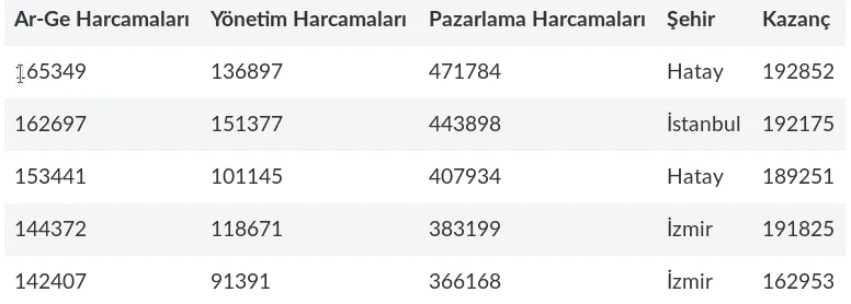
In the application we will build, we know the R&D spending, administration spending and marketing spending of some software companies in various cities in Turkey, which city they are in, and their profit. What we want to do is find which of these variables relate to profit and make predictions around that. You can build on the dataset below, put it into dataset format as a csv file, and use it with your Python code.

I am sharing the code we ended up with in the preprocessing post again below.

#Adding the libraries
import numpy as np
import matplotlib.pyplot as plt
import pandas as pd

#Adding the dataset
dataset = pd.read_csv('Data.csv')

#Taking every column except the last one into a new object array, meaning city, age and salary.
X = dataset.iloc[:, :-1].values

#Assigning the last column into an object array
y = dataset.iloc[:, 4].values

#Turning the categorical data in the city column into numbers
from sklearn.preprocessing import LabelEncoder
labelencoder_X = LabelEncoder()
labelencoded_sehir=labelencoder_X.fit_transform(X[:, 3])

# Splitting the independent variable object array (X) and the dependent variable object array (y) of the dataset separately into a training set and a test set

from sklearn.model_selection import train_test_split
X_train, X_test, y_train, y_test = train_test_split(X, y, test_size = 0.2, random_state = 0)

# The linear regression equation
from sklearn.linear_model import LinearRegression
regressor = LinearRegression()
regressor.fit(X_train, y_train)

# Predicting the test results
y_pred = regressor.predict(X_test)

In multiple linear regression, the only thing we have to do before running this code is to work out with the elimination methods which variables are needed, and build a dataset that contains only those.

This post got a bit long, but it was one of the longest topics. Thank you for reading it patiently.

Good luck, and stay well.

Abdullah Faruk ÇİFTLER