Data Science Notes 3: Data preprocessing

Hello. In this post we will look for answers to questions like what data preprocessing is and what kind of operations it involves. Enjoy the read.

Before saying what preprocessing is, I want to say why it is needed. Let us use the dataset we talked about in the first post. Imagine we have a dataset with the properties listed below:

• Data missing or lost in some rows. For example, in a system that records the temperature and humidity of a district as one row per second, some rows have only humidity, some have only temperature, and some have neither.
• Values with strong anomalies arriving one after another in absurd ways. For instance numbers running 2, 3, 5, 6 and then suddenly 140 or 1400. Or a power line whose voltage normally moves between 220 and 240 showing around 10000 for a second.

Situations like the ones above are the ones that damage a machine learning algorithm. They most likely come from a fault in the measuring device or in the method. So when we train the machine learning software we write, we have to make sure it does not take these values into account. By minimising these unwanted cases through preprocessing, we can make the most accurate analysis. Preprocessing is a wide topic, but for now I will pass on my notes about filling in missing values, turning categorical attributes into numbers and feature scaling. I will close the post by covering the test set and training set I mentioned in the first post. I will add to it over time as needed.

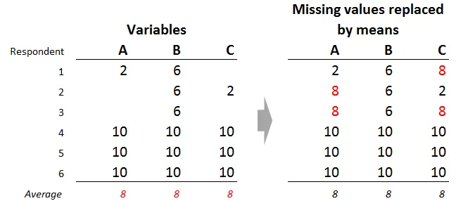
Filling missing values with the mean

As I mentioned above, in some datasets part of the data can be missing because of gaps in the measurement or flaws in the collection method. To make up for it there are methods such as filling with the mean value and filling with the most likely value. In this post we will see filling missing values with the mean. For every operation in this post we will use the data in the table below, pulled from the “Data.csv” file, as our example dataset. If you look carefully at the table you will see that some values are missing.

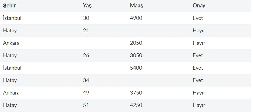
Before any of this, we need to load Data.csv and the required libraries into Python as described in the previous post. I have added it again in the example below.

#Adding the libraries
import numpy as np
import matplotlib.pyplot as plt
import pandas as pd

#Adding the dataset
dataset = pd.read_csv('Data.csv')

#Setting the missing values to the mean of all values in the same variable
dataset["Yaş"].fillna(dataset["Yaş"].mean(), inplace=True)
dataset["Maaş"].fillna(dataset["Maaş"].mean(), inplace=True)

#Taking every column except the last one into a new object array, meaning city, age and salary.
X = dataset.iloc[:, :-1].values

#Assigning the last column into an object array
y = dataset.iloc[:, 3].values

Once we run all of this, the missing values in our table are replaced by the mean of that column, as shown below.

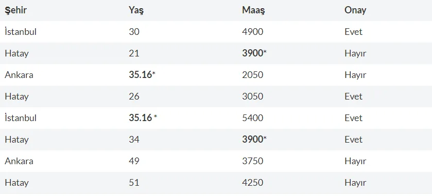
.iloc: finds a column by its index. In other words, using ‘iloc’ lets us take columns by index alone.

.values: returns the values of the columns you took (by index) inside a NumPy array. That is basically how X and y become NumPy arrays.

Turning categorical attributes into numbers

Turning categorical data into numbers is required for a machine learning algorithm to run at all, because every mathematical operation is done on numeric variables. In the previous example we assigned every column except the “Onay” column into the X object array. So inside X only the city stayed categorical and everything else was numeric. If we want to run an analysis on X, the city column is the one we have to make numeric.

#Turning the categorical data in the city column into numbers
from sklearn.preprocessing import LabelEncoder
labelencoder_X = LabelEncoder()
labelencoded_sehir=labelencoder_X.fit_transform(X[:, 0])

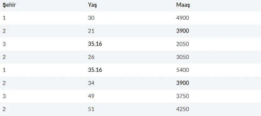
When we add the code above to the rest of our code, we get an object array like the one below. You will see that Istanbul is assigned the number 1, Hatay 2 and Ankara 3. We will understand the main reason for this better when we get to the types of regression.

Splitting the dataset into a training set and a test set

I am bringing the heading from my first post here again to remind you of the situation, and then I will try to explain how it is done.

Why are datasets split?

Here is one way to explain it. Say we have twelve months of weather data and we want to build a forecasting application with it to predict future weather. Machine learning algorithms need data to train themselves. You can think of it like this. Your view of a city forms through the people you already know who are from there. You more or less know what those people are like. A machine learning application asks us for data about people from that city so it can form a picture of them.

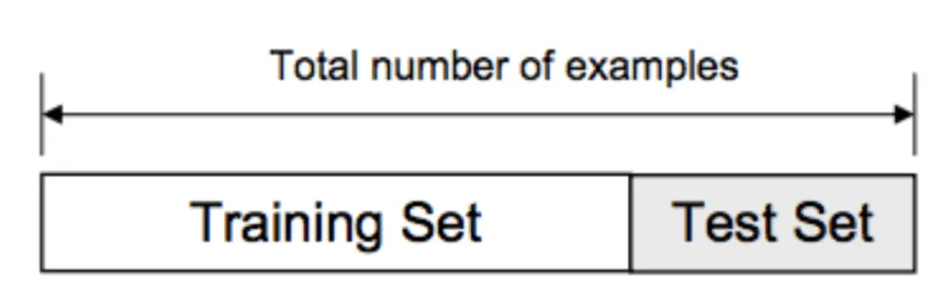
That is not the end of it. Our data is limited and we have to test whether the algorithm works correctly. Say we gave the algorithm the data of every person from Hatay that we know. Now we have no people left to test whether it works. So we split our data in two. We give part of it so the algorithm gets to know people from Hatay, and we keep the rest to test whether it works. Datasets are generally split in two.

Training set: the set built so the machine learning algorithm can get to know the data and make its predictions on it during training. In short, the dataset that makes it biased in certain ways towards the data that comes next.

Test set: the dataset we set aside earlier to test how correctly the algorithm built from the training set works.

# Splitting the independent variable object array (X) and the dependent variable object array (y) of the dataset separately into a training set and a test set

from sklearn.model_selection import train_test_split
X_train, X_test, y_train, y_test = train_test_split(X, y, test_size = 0.2, random_state = 0)

test_size: this is where we set the ratio between the training set and the test set. In this example, for every 10 records it sends 2 to the test set and 8 to the training set. The test set is usually 0.2, because having plenty of data matters for training the model correctly. We can test accuracy with little data, but we cannot train a model with little data.

All the preprocessing code

#Adding the libraries
import numpy as np
import matplotlib.pyplot as plt
import pandas as pd

#Adding the dataset
dataset = pd.read_csv('Data.csv')

#Setting the missing values to the mean of all values in the same variable
dataset["Yaş"].fillna(dataset["Yaş"].mean(), inplace=True)
dataset["Maaş"].fillna(dataset["Maaş"].mean(), inplace=True)

#Taking every column except the last one into a new object array, meaning city, age and salary.
X = dataset.iloc[:, :-1].values

#Assigning the last column into an object array
y = dataset.iloc[:, 3].values

#Turning the categorical data in the city column into numbers
from sklearn.preprocessing import LabelEncoder
labelencoder_X = LabelEncoder()
labelencoded_sehir=labelencoder_X.fit_transform(X[:, 0])

# Splitting the independent variable object array (X) and the dependent variable object array (y) of the dataset separately into a training set and a test set

from sklearn.model_selection import train_test_split
X_train, X_test, y_train, y_test = train_test_split(X, y, test_size = 0.2, random_state = 0)

In the next post I will look for answers to questions like what feature scaling is and why it matters. After that we will move on to the types of regression.

Good luck with it.

Abdullah Faruk ÇİFTLER