Data Science Notes 8: Support vector regression

My earlier posts in this series:

• Data Science Notes 1, Introduction to machine learning
• Data Science Notes 2, Machine learning and Python
• Data Science Notes 3, Data preprocessing
• Data Science Notes 4, Feature scaling
• Data Science Notes 5, Linear regression
• Data Science Notes 6, Multiple linear regression
• Data Science Notes 7, Polynomial regression

Hello,

In this post I will share the notes I took while studying support vector regression. I hope they are useful.

An introduction to support vector regression

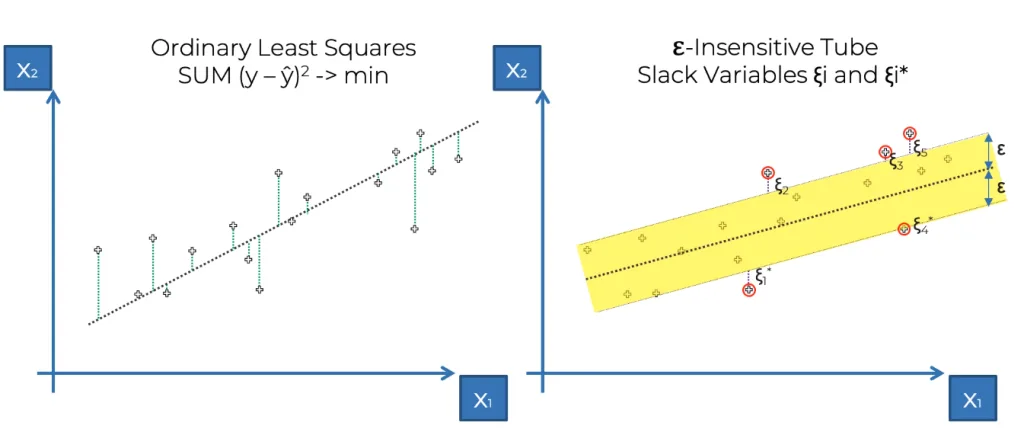
Before getting into support vector regression, let us briefly recall linear regression and the least squares method. If you want to read it in more detail you can go to the linear regression post. In short, the least squares method in linear regression means drawing a line on a plane of data points such that the sum of the squared distances from that line to all the points is lower than for any other line you could draw. It sounds tangled written out like this, so as I said you can lean on the linear regression post. There is a fairly detailed explanation there.

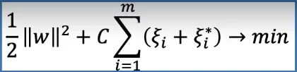
In support vector regression things work a little differently. The most basic difference between linear regression and support vector regression is that linear regression takes every point in the training set into account, while support vector regression takes points into account according to a parameter. That parameter is that the points to be counted have to be at least epsilon away from the regression line that will be built. As you see above, points that are not at epsilon distance are not taken into account in support vector regression. How the epsilon distance is decided is put into a formula below.

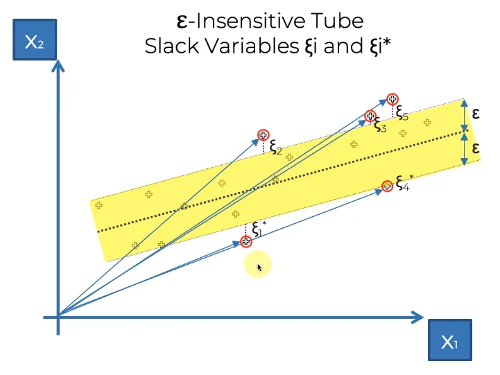
So why is this algorithm called support vector regression? The main reason is that each of the points outside epsilon forms a vector starting from the origin of the system. We see this in detail below.

As in every post, we will work through a problem here. Our problem will be exactly the same as the one in the previous lesson on polynomial regression. That way we also get a performance comparison between the two types of regression. Let us recall it:

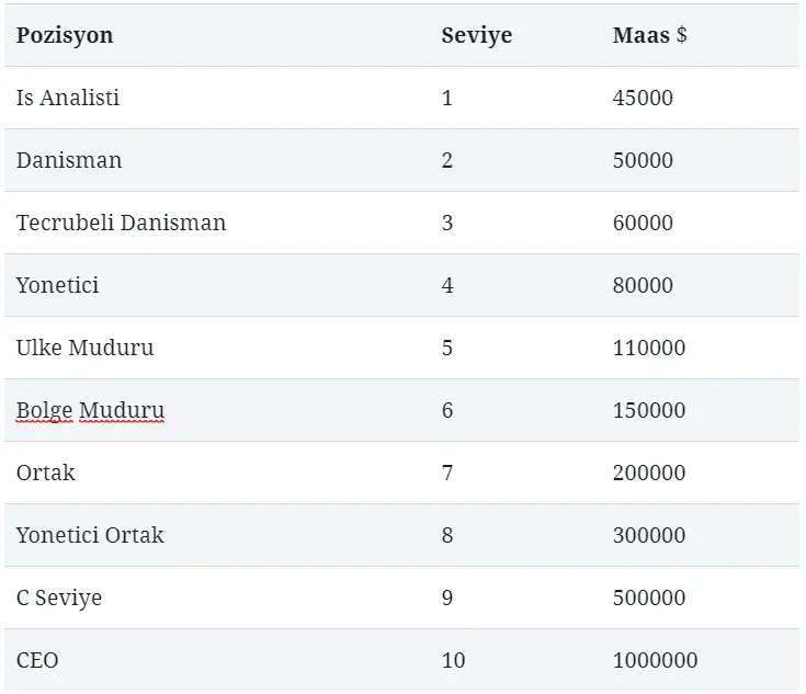
We have a dataset of salaries by position level. In the previous lesson we built our polynomial regression model from this dataset. In this lesson we will take the same problem and try to model the same dataset with support vector regression.

The Python application

# Adding the libraries
import numpy as np
import matplotlib.pyplot as plt
import pandas as pd

# Adding our dataset and splitting it into training and test sets
dataset = pd.read_csv('maas.csv')
X = dataset.iloc[:, 1:-1].values
y = dataset.iloc[:, -1].values
print(X)
print(y)
y = y.reshape(len(y),1)
print(y)

# Applying feature scaling
from sklearn.preprocessing import StandardScaler
sc_X = StandardScaler()
sc_y = StandardScaler()
X = sc_X.fit_transform(X)
y = sc_y.fit_transform(y)
print(X)
print(y)

# Training the dataset as an SVR model
from sklearn.svm import SVR
regressor = SVR(kernel = 'rbf')
regressor.fit(X, y)

# Making a new prediction.
sc_y.inverse_transform(regressor.predict(sc_X.transform([[6.5]])))

# Visualising the SVR results
plt.scatter(sc_X.inverse_transform(X), sc_y.inverse_transform(y), color = 'red')
plt.plot(sc_X.inverse_transform(X), sc_y.inverse_transform(regressor.predict(X)), color = 'blue')
plt.title('Truth or Bluff (SVR)')
plt.xlabel('Position level')
plt.ylabel('Salary')
plt.show()

# Showing the SVR results in more detail.
X_grid = np.arange(min(sc_X.inverse_transform(X)), max(sc_X.inverse_transform(X)), 0.1)
X_grid = X_grid.reshape((len(X_grid), 1))
plt.scatter(sc_X.inverse_transform(X), sc_y.inverse_transform(y), color = 'red')
plt.plot(X_grid, sc_y.inverse_transform(regressor.predict(sc_X.transform(X_grid))), color = 'blue')
plt.title('Truth or Bluff (SVR)')
plt.xlabel('Position level')
plt.ylabel('Salary')
plt.show()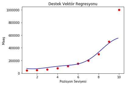

Looking at the result chart above, we see that support vector regression is not very useful for values that are not stable. For the dataset we used as an example here, the polynomial regression we applied in the previous lesson returns far better results. In later lessons we will look at the performance of the regression types in much more detail, and talk about which regression model to pick for which kind of dataset and problem.

EXTRA

I think it will stay with you longer if you do a short search on Vladimir Vapnik, who invented support vector regression, and find what he worked on. Later on, when we get to support vector machines, we will also touch on non linear support vector regression.

If there is anything you did not understand, feel free to ask. Thank you very much for reading this far.

See you in the next lesson.

Stay well.