Data Science Notes 5: Linear regression

All the statistics in the world can’t measure the warmth of a smile.

My earlier posts in this series:

Data Science Notes 1, Introduction to machine learning

Data Science Notes 2, Machine learning and Python

Data Science Notes 3, Data preprocessing

Data Science Notes 4, Feature scaling

The idea of regression

With this post we start on the types of regression. Before getting into linear regression I want to say what regression means. Regression is basically the way we express the function between variables mathematically. In other words, it is putting the relationships between two (or more) different arguments into a formula.

Simple linear regression

Chart No.1

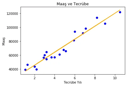
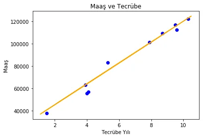
It is an analysis method modelled as a straight line that relates inputs to outputs. It splits into two, simple linear regression and multiple linear regression. As you see in the example above, the relationship between salary and experience has been analysed with linear regression. There is clearly a linear ratio between years of experience and salary. Let me explain this in more detail and then come back to the picture above. I numbered the charts so we do not mix them up, and you can follow the post by watching the figure, picture and chart numbers. After going through linear regression on a definitional chart, we will come back to Chart No.1.

Chart No.2

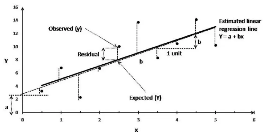
Looking at the chart above we see several concepts. Let me explain them one by one and then move to the practical part.

Y: the values predicted by the linear regression model, which form a straight line when ordered.

a= the starting variable inside the equation. In Chart No.1 it stands for the number 40000.

Expected(Y): the value the linear regression model predicts. Say someone with one year of experience at a company earns 4000 lira. Someone with three years at the same company earns 12000 lira. From this dataset the linear regression model predicts the salary of someone with two years as 8000 lira. In reality people with two years of experience at that company might earn 9000 lira. Expected Y shows us the predictions of the linear regression model.

Observed(y): this is the value in the test set for the predicted data point, not the predicted value itself.

Residual: the residual is exactly the difference between the real value in the test set and the value our linear regression model predicted. So we can call it the distance of the real value from the regression value, in other words the margin of error.

Linear Regression Line: the regression line on which the values predicted by the model (the Expected Y values) sit.

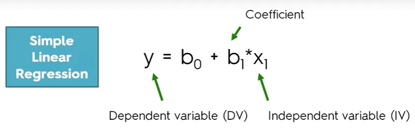
Looking at the linear regression equation we see that y is the dependent variable and x1 is the independent variable.

To explain the terms dependent and independent variable, going back to Chart No.1 is enough. In that chart it is clear that the salary changes as the years of experience change. The kind of variable we want to predict, the one that changes when we change certain other variables, meaning salary here, is what we call the independent variable. The dependent variables are all the variables that appear in the formula and affect the change when the change of the independent variable is written out. Years of experience, the single independent variable in Chart No.1, works this way.

The least squares method

We can say the least squares method is the most basic idea in linear regression. The whole algorithm is built on it. Let us look at what it is. If we look at the residual in Chart No.2, the distance between the value predicted by the linear regression model and the real value in the test set, we see that it is really the margin of error of our prediction. Now think of it this way: if every predicted value has a residual, and that residual runs from 0 (which means the predicted value is the same as the real one, congratulations) to infinity, then summing the squares of the residuals of all our predictions gives us a number that corresponds to the total error. We have to square them because the residual is negative when the real value is lower than the predicted one. So we should build a linear regression model that draws a line which minimises the residuals, meaning the line that gives us the smallest total error.

The Python application

First let us create a csv file like the table below.

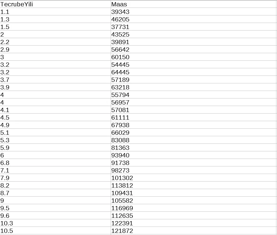
Then let us write the Python code below into our editor.

#Adding the libraries
import numpy as np
import matplotlib.pyplot as plt
import pandas as pd

#Adding the dataset
dataset = pd.read_csv('maasverisi.csv')
X = dataset.iloc[:, :-1].values
y = dataset.iloc[:, 1].values

# Splitting the independent variable object array (X) and the dependent variable object array (y) of the dataset separately into a training set and a test set
from sklearn.model_selection import train_test_split
X_train, X_test, y_train, y_test = train_test_split(X, y, test_size = 1/3, random_state = 0)

#Training the linear regression model on the training set
from sklearn.linear_model import LinearRegression
regressor = LinearRegression()
regressor.fit(X_train,y_train)

#Making predictions on the test set
y_pred = regressor.predict(X_test)
#Visualising the test results
plt.scatter(X_test, y_test, color ='blue')
plt.plot(X_train, regressor.predict(X_train), color='orange')
plt.title('Maaş ve Tecrübe')
plt.xlabel('Tecrübe Yılı')
plt.ylabel('Maaş')
plt.show()

The result we get looks like this.

In this post we looked for answers to what simple linear regression is and what the least squares method is. I hope it was useful. See you in the multiple linear regression post.

Good luck with it.

Abdullah Faruk ÇİFTLER